The Value Inversion

The Reversal of the Price-to-Sales Ratio

For the past few years, investors have noticed what we call a “value inversion,” which appears to be getting progressively worse. The chart below exemplifies what’s happening:

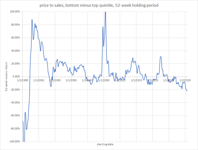
Theoretically—and normally—stocks with low price-to-sales ratios (cheap stocks) outperform those with high price-to-sales ratios (expensive stocks). As you can see from the above chart, such was the case over the majority of the current century, and indeed, as James O’Shaughnessy has shown in What Works on Wall Street, for most of the twentieth century too.

But things began to change in 2014. Between January 1, 2014 and today, if you had invested in the lowest quintile of price-to-sales stocks, with monthly rebalancing and ignoring transaction costs, you would have lost 24.08% of your money; if you had invested in stocks with the highest price-to-sales ratio during that period, you would have made a profit of 40.23%. That’s an astonishing 64-point difference. There have been periods of value inversion before, but I don’t think there’s ever been one this long and this severe.

Here are two bar charts documenting the same phenomenon:

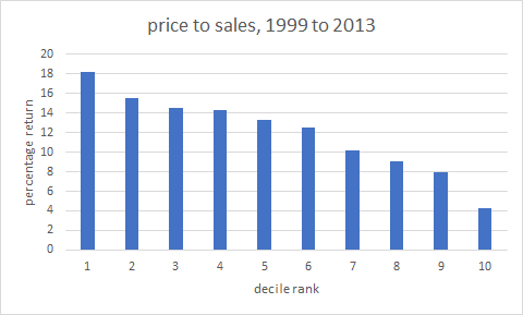
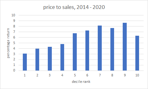
In this article I want to dig deep and investigate how widespread the value inversion has been since 2014, and how a smart investor might deal with it going forward.

Skip This Section If You Don’t Care About the Technical Details of the Measurements I’m Using

All data is from Portfolio123. I’m using a universe of stocks with a minimum market cap of $100 million, a minimum median daily dollar volume of $100,000, and a minimum price of $1.00; I am including ADRs and Canadian stocks that can be traded in the US. When I use enterprise value–based ratios, I exclude stocks in the financial and real estate sectors. All returns are based on investing in quantiles according to the factor every four weeks and holding for fifty-two weeks. The line charts subtract the top quintile from the bottom in the case of price-to-X ratios and the bottom quintile from the top in the case of yield ratios. The bar decile charts are the averages of the 52-week returns over the periods 1/1/1999 to 1/1/2014 and 1/1/2014 to 4/25/2020. For the price-to-X ratios, companies with negative values for earnings, EBITDA, book value, or free cash flow were excluded from the universe, as is conventional. Comparing the performance of the top quintile to the bottom quintile has been a standard measure of success or failure of a factor for many decades. It is far from perfect: ignoring the middle three quintiles is questionable at best, and the entirety of the distribution should ideally be considered. This is why I’ve supplemented these timelines with decile bar charts.

The Failure of Other Conventional Value Metrics

Below are the same charts but using different value metrics.

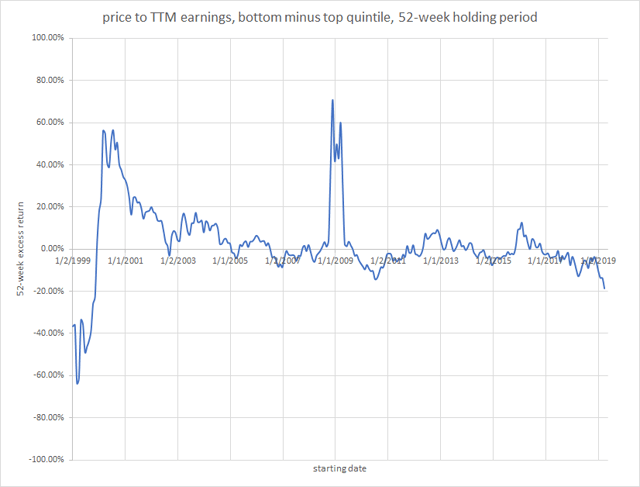
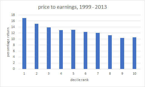
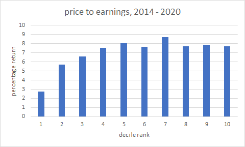
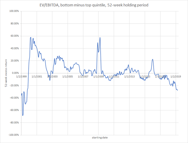
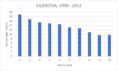
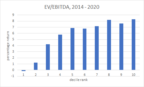
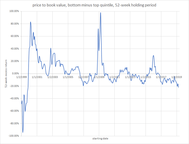
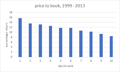
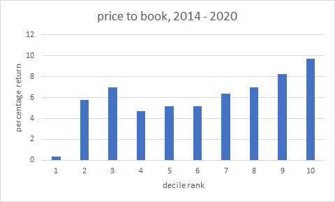
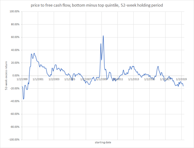
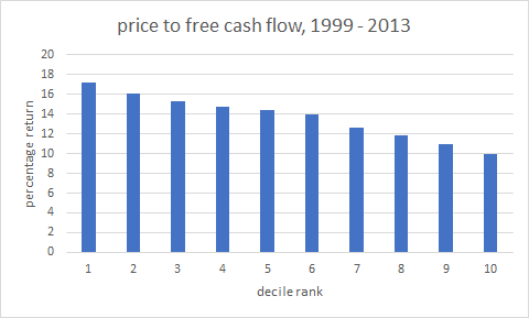
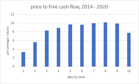
Clearly, all of these very conventional and widely used value ratios have stopped working (or are working backwards). Most of them stopped working around 2014, but price to book value seems to have stopped working earlier. Whether this is temporary or permanent is the question we must address.

The Possible Reasons for the Failures

I can think of three possible reasons for the failure of these ratios over the last six years.

1. Investors are no longer considering the price of their investments.
2. Investors are deliberately choosing to invest in high-priced stocks and shunning cheap stocks.
3. Investors are still considering the price of their investments but these five ratios are inadequate measures of value because of overuse.

I will withhold judgment on the first and second reasons. Certainly a lot of investors have been buying stocks without looking at their prices, basing their decisions on FOMO or momentum or popularity or fad. On the other hand, there are plenty of value-minded investors out there too.

The third reason depends on the theory of arbitrage. To quote from Charles M. C. Lee and Eric So’s book Alphanomics, the conventional economic view is that “If a particular piece of value-relevant information is not incorporated into price, there will be powerful economic incentives to uncover it, and trade on it. As a result of these arbitrage forces, price will adjust to fully reflect the information. . . . Faith in the efficacy of this mechanism is a cornerstone of modern financial economics.”

We can put it another way. Maybe by 2014, algorithmic valuation models had come to dominate the world of investing, and the five value formulas that were used by these valuation models were price to sales, price to book, price to earnings, price to free cash flow, and EV/EBITDA. It would be entirely logical, then, that through the process of arbitrage these formulas would fail to predict price movements.

How would this work in practice? Let’s say that a very large number of investors were buying stocks with price-to-book values of less than the median. The prices of those stocks would then rise until they were close to the median. The stocks that now had the lowest price-to-book ratios would be stocks that for one reason or another were remarkably undesirable stocks. In other words, these are stocks that deserved a low price-to-book ratio. The arbitrage mechanism would have worked.

If this were to happen with every single one of these formulas, the cheap-looking stocks would appear deservedly cheap because they were unattractive investments and the expensive-looking stocks would appear deservedly expensive because they were attractive investments. And that’s the kind of market that we seem to be in at the moment.

Proving the Case for Arbitrage

Let’s say that there are certain metrics for valuing stocks that are not widely used and therefore have not been arbitraged. If we look at the results of these metrics by the same measure as we’ve just used for the big five—best quintile minus worst quintile over time—we’ll see one of three things happening.

1. The metrics will be useless. They will work sometimes and not other times and no conclusions can be drawn.
2. The metrics will show the same pattern as the big five: they will work prior to 2014 and not afterwards.
3. The metrics will show persistence both before and beyond 2014.

If we actually see number three, then that will demonstrate that value is not dead but that instead the conventional measures of value have simply been arbitraged away. But if we see only numbers one and two, then we may have to conclude that value, as a factor, is, if not dead, at least in an extended state of hibernation.

So I’m now going to show you some charts based on three other measures of value. All of these are structured as “yield” ratios—i.e. the price is in the denominator rather than the numerator, so we’re looking at highest quintile minus lowest. This difference can be purely cosmetic—all of the above quintile charts would have looked exactly the same if I’d used, say, EBITDA/EV rather than EV/EBITDA and excluded companies with negative EBITDAs from the top and bottom quintiles, and all of the decile charts would be mirror images of the ones above. But when you use yield-based formulas you don’t exclude companies with negative earnings or free cash flow. Instead they go in the bottom quantile(s) and companies with strong earnings, free cash flow, and so on are in the top.

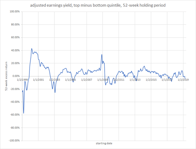
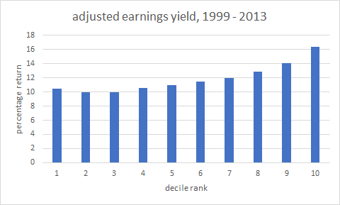
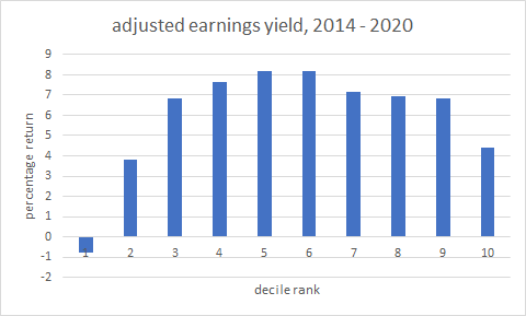
This ratio takes the TTM net income, adjusts it for special items, divides it by market cap, and compares the result to other companies in the same industry.

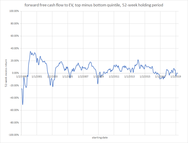
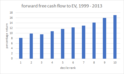
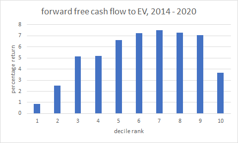
This is the current year’s free cash flow estimate divided by enterprise value and compared to other companies in the same sector; where the estimate is not available I use TTM unlevered free cash flow instead. This is a short-term version of the ratio analysts use for discounted cash flow analysis.

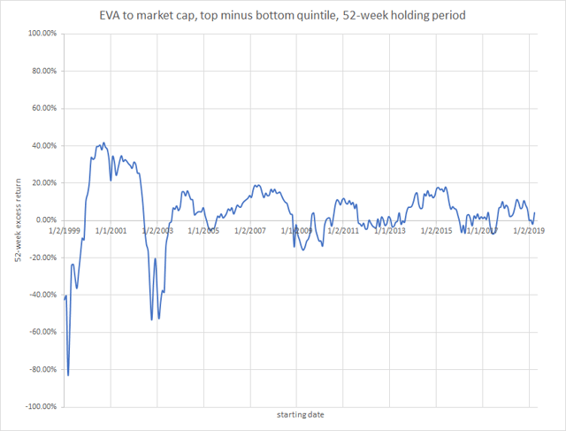
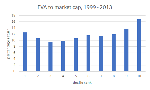
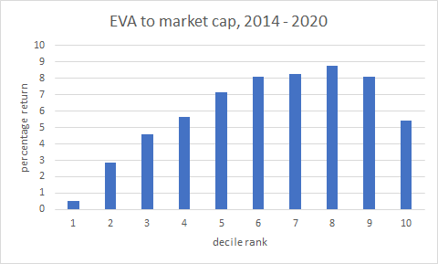
EVA stands for economic value added, a measure Joel Stern came up with in the 1960s. Essentially it’s the net operating profit after taxes minus the product of the weighted average cost of capital and the economic assets employed. I divide that by the company’s market cap.

With these metrics (the first two are quite commonly used, the third has been largely forgotten), there has clearly been a recent diminution in the degree to which the top quintile exceeds the bottom quintile. But, significantly, there has been no real value inversion. The ratios may be less effective now, but they still work.

Why Alternative Value Metrics Still Work

Are these metrics better, then, than the widely used ones?

I would argue that they are, arbitrage or not. The first, earnings yield compared to industry, is very similar to the p/e ratio, but the p/e ratio is conventionally compared to all other companies, regardless of industry. The top quintile of the p/e ratio is occupied by companies with low but not negative earnings, while the bottom quintile of the earnings yield is occupied by companies with negative earnings. If you don’t rank those, your results will never be very reflective of what a difference earnings can make.

The second and third metrics were both invented by Joel Stern, one of the most brilliant and original thinkers the financial world has produced. Stern came up with free cash flow (as opposed to just cash flow) in 1972, introducing the idea of deducting capital expenditures from operating cash flow, which quickly became the standard way to measure it for discounted cash flow valuation models. His work with EVA made him one of the most valued business consultants in the country. Both measures give a far more holistic perspective of a company than do the others. Significantly, both are close to fifty years old, so they’re not newfangled measures.

The reason that forward free cash flow to EV works better than free cash flow to price is fourfold. First, companies with negative free cash flow were excluded in the first measure and included in the second. Second, free cash flow to price has, arguably, been subject to more arbitrage. Third, the measure I’m using compares companies in the same sector rather than the entire universe. I do this so that sectors with typically low free cash flow, such as utilities, don’t get punished. And fourth, enterprise value allows one to consider the entirety of a company’s value rather than only the value of its equity, and free cash flow is generated by the entirety of a company’s capital, not only its equity.

Is the Value Inversion Real?

Considering that the value inversion seems to be occurring if you use common metrics in an unsophisticated manner but not if you use well-established and sensible metrics in a sophisticated manner, is it real?

The very first chart in this article, the one that shows the performance of the price-to-sales ratio, seems to indicate that the value inversion is truly real. Even if we were to change our measure to compare stocks within the same industry, you’d see a rather drastic reversal in the last three years.

But if we consider the price-to-sales ratio a fully arbitraged factor, perhaps the value inversion is only a statistical artifact, a proof of the workings of arbitrage. Perhaps price still matters. We just need to compare it to something more sophisticated than the top line of the income statement.

How to Invest During an Apparent Value Inversion

Valuing a company is hard work. I think the charts for the first five ratios will show that simplistic methods are no longer working because they’ve been overused. To get at a company’s true value requires more than a simple ratio. Ideally, one should look at every aspect of a company’s business, from its cash conversion cycle to its net operating assets, from its earnings growth to its free cash flow return on assets, from its margins to its moat. No one number is going to capture a company’s value.

In addition, stock prices rise and fall not because a company’s value changes but because investor estimations of a company’s value change. The key to successful investing lies in anticipating these changes. When we call a company overvalued or undervalued, we should be thinking not of what the company is really worth but what investors think it will be worth in the future. Doing so means looking at its prospects for growth, which are in turn determined by all those aspects of its business I listed above along with a large number of things that are harder or impossible to measure. And we don’t want to invest in companies with the highest growth prospects. We want to invest in companies that we think have prospects that are higher than those that the market already thinks they have—in other words, companies that will surprise investors.

It’s a complicated dance. Because of the prevalence of index funds and algorithms that choose stocks based on elementary value criteria, a company no longer has a built-in advantage if its price-to-sales or EV/EBITDA ratio is low. It’s even possible to imagine a world in which every factor one can suss out from a company’s financials has been fully arbitraged.

Thankfully, we’re not quite there yet.

What about the value factors that seem to have been arbitraged? Will they begin working again at some point?

It’s entirely possible. After all, the price to earnings ratio has been in use at least since the 1920s and, depending on how it’s used, it still works. I, for one, still use many of these ratios. But not as much as I used to.